DISCLAIMER
The present benchmark was conducted on 2025-06-11 on a Macbook Pro M4
(12-core CPU, 16-core GPU, 24GB RAM). Results will vary
depending on the hardware. The benchmarks are intended to provide a
general idea of the performance differences between the fio
package and other implementations, but they should not be considered
definitive. The performance of the functions may also vary depending on
the specific data used and the context in which the functions are
applied.
Introduction
This vignette presents a benchmarking analysis comparing the
performance of functions from the fio package with
equivalent base R functions. The fio package provides a set
of functions for input-output analysis, a method used in economics to
analyze the interdependencies between different sectors of an
economy.
In this document, we will focus on two key functions: the technical coefficients matrix calculation and the Leontief inverse matrix calculation. These functions are fundamental to input-output analysis, and their performance can significantly impact the speed of larger analyses.
Our benchmarking tests, which involve running these functions
repeatedely in simulated datasets, show that the fio
package functions are faster than other implementations. This improved
performance can make a substantial difference in larger analyses, making
the fio package a valuable tool for input-output analysis
in R.
The tests were run on a simulated matrix, and each test was repeated 100 times to account for variability. Please note that the results of this benchmarking analysis are dependent on the specific test datasets used and the hardware on which the algorithms were run. Therefore, the results should be interpreted in the context of these specific conditions.
Technical coefficients matrix
The technical coefficients matrix calculation, a key and initial step
in input-output analysis, was tested using the
compute_tech_coeff() function from the fio
package, equivalent functions from the leontief package,
and a base R implementation. It consists on dividing each
element of intermediate transactions matrix by the correspondent
element of total production vector1.
# set seed
set.seed(100)

# Base R function
tech_coeff_r <- function(intermediate_transactions, total_production) {
  tech_coeff_matrix <- intermediate_transactions %*% diag(1 / as.vector(total_production))
  return(tech_coeff_matrix)
}

# benchmark
benchmark_a <- bench::press(
  matrix_dim = c(100, 500, 1000, 2000),
  {
    intermediate_transactions <- matrix(
      as.double(sample(1:1000, matrix_dim^2, replace = TRUE)),
      nrow = matrix_dim,
      ncol = matrix_dim
    )
    total_production <- matrix(
      as.double(sample(4000000:6000000, matrix_dim, replace = TRUE)),
      nrow = 1,
      ncol = matrix_dim
    )
    iom_fio <- fio::iom$new("iom", intermediate_transactions, total_production)
    bench::mark(
      fio = fio:::compute_tech_coeff(intermediate_transactions, total_production),
      `Base R` = tech_coeff_r(intermediate_transactions, total_production),
      leontief = leontief::input_requirement(intermediate_transactions, total_production),
      iterations = 100
    )
  }
)
#> Running with:
#>   matrix_dim
#> 1        100
#> 2        500
#> 3       1000
#> 4       2000
#> Warning: Some expressions had a GC in every iteration; so filtering is
#> disabled.
print(benchmark_a)
#> # A tibble: 12 × 14
#>    expression matrix_dim      min   median `itr/sec` mem_alloc `gc/sec` n_itr
#>    <bch:expr>      <dbl> <bch:tm> <bch:tm>     <dbl> <bch:byt>    <dbl> <int>
#>  1 fio               100  49.57µs  81.41µs   11381.   861.83KB     0      100
#>  2 Base R            100  59.61µs  78.72µs   11191.   190.65KB     0      100
#>  3 leontief          100 131.45µs 161.95µs    6175.   706.38KB    62.4     99
#>  4 fio               500 445.67µs 625.95µs    1562.     1.91MB    65.1     96
#>  5 Base R            500 940.38µs   1.27ms     722.     3.82MB    80.2     90
#>  6 leontief          500   1.73ms   2.11ms     464.    16.29MB   691.      41
#>  7 fio              1000   1.83ms   2.38ms     405.     7.63MB    83.0     83
#>  8 Base R           1000   6.56ms   7.88ms     125.    15.27MB    70.1     64
#>  9 leontief         1000   8.46ms    8.6ms     116.       65MB  9131.       2
#> 10 fio              2000   9.56ms  10.89ms      87.9   30.52MB    12.3    100
#> 11 Base R           2000  45.27ms  52.44ms      18.8   61.05MB     6.38   100
#> 12 leontief         2000  39.91ms  62.49ms      16.4   259.7MB    44.6    100
#> # ℹ 6 more variables: n_gc <dbl>, total_time <bch:tm>, result <list>,
#> #   memory <list>, time <list>, gc <list>

# plot
ggplot2::autoplot(benchmark_a)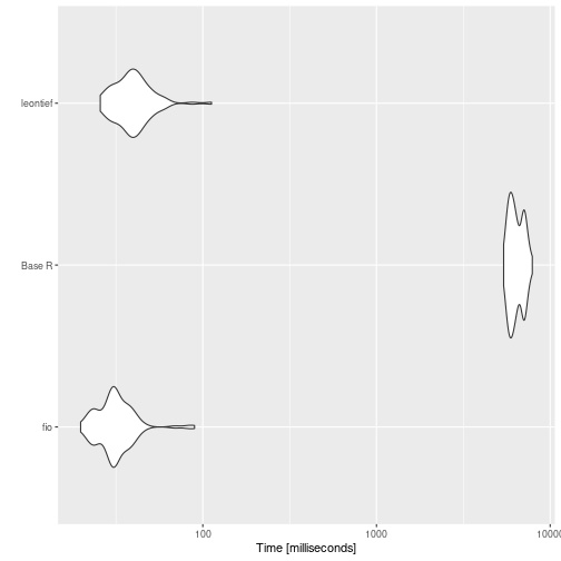
is faster.
Leontief inverse matrix
When we’re talking about inverting a there’s a lot more work involved. Leontief matrix () is obtained from subtracting the technical coefficients matrix () from the identity matrix (), therefore it has no null rows or columns.
It allows for solving the linear system through LU decomposition, which is a more efficient method than the direct inverse matrix calculation.
# base R function
leontief_inverse_r <- function(technical_coefficients_matrix) {
  dim <- nrow(technical_coefficients_matrix)
  leontief_inverse_matrix <- solve(diag(dim) - technical_coefficients_matrix)
  return(leontief_inverse_matrix)
}

# benchmark
benchmark_b <- bench::press(
  matrix_dim = c(100, 500, 1000, 2000),
  {
    intermediate_transactions <- matrix(
      as.double(sample(1:1000, matrix_dim^2, replace = TRUE)),
      nrow = matrix_dim,
      ncol = matrix_dim
    )
    total_production <- matrix(
      as.double(sample(4000000:6000000, matrix_dim, replace = TRUE)),
      nrow = 1,
      ncol = matrix_dim
    )
    iom_fio <- fio::iom$new("iom", intermediate_transactions, total_production)
    iom_fio$compute_tech_coeff()
    technical_coefficients_matrix <- iom_fio$technical_coefficients_matrix
    bench::mark(
      fio = fio:::compute_leontief_inverse(technical_coefficients_matrix),
      `Base R` = leontief_inverse_r(technical_coefficients_matrix),
      leontief = leontief::leontief_inverse(technical_coefficients_matrix),
      iterations = 100,
      check = FALSE
    )
  }
)
#> Running with:
#>   matrix_dim
#> 1        100
#> 2        500
#> 3       1000
#> 4       2000
#> Warning: Some expressions had a GC in every iteration; so filtering is
#> disabled.
print(benchmark_b)
#> # A tibble: 12 × 14
#>    expression matrix_dim      min   median `itr/sec` mem_alloc `gc/sec` n_itr
#>    <bch:expr>      <dbl> <bch:tm> <bch:tm>     <dbl> <bch:byt>    <dbl> <int>
#>  1 fio               100 138.58µs  339.4µs   2410.    158.51KB     0      100
#>  2 Base R            100 254.04µs 356.86µs   2765.    413.27KB     0      100
#>  3 leontief          100 270.72µs  363.4µs   2837.    402.57KB     0      100
#>  4 fio               500   4.83ms   5.78ms    172.      3.81MB     3.51    98
#>  5 Base R            500   3.96ms   4.27ms    230.      9.55MB    20.0     92
#>  6 leontief          500   3.99ms   4.26ms    231.      9.55MB    20.1     92
#>  7 fio              1000  24.13ms  27.31ms     36.6    15.26MB     3.62    91
#>  8 Base R           1000  16.67ms  17.36ms     56.8    38.18MB    16.0     78
#>  9 leontief         1000  15.96ms   17.3ms     57.3    38.18MB    16.2     78
#> 10 fio              2000 129.76ms 136.91ms      7.26   61.03MB     1.45   100
#> 11 Base R           2000  85.67ms  89.92ms     10.9   152.66MB    11.1    100
#> 12 leontief         2000  85.94ms  90.43ms     10.8   152.66MB    10.8    100
#> # ℹ 6 more variables: n_gc <dbl>, total_time <bch:tm>, result <list>,
#> #   memory <list>, time <list>, gc <list>

# plot
ggplot2::autoplot(benchmark_b)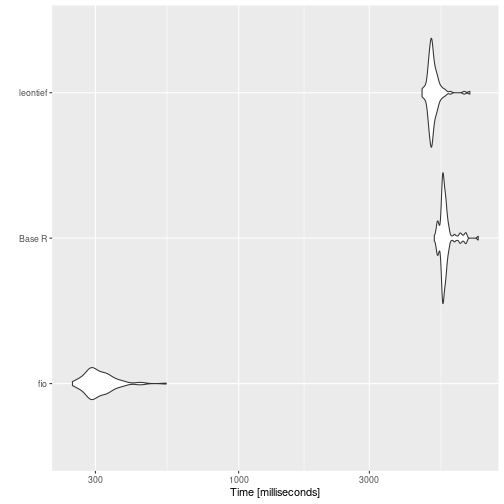
{fio} is incredibly faster.
Sensitivity of dispersion coefficients of variation
To represent linkage-based functions performance, we compute benchmark for sensitivity of dispersion coefficients of variation.
# base R function
sensitivity_r <- function(B) {
  n <- nrow(B)
  SL = rowSums(B)
  ML = SL / n
  (((1 / (n - 1)) * (colSums((B - ML) ** 2))) ** 0.5) / ML
}

# benchmark
benchmark_c <- bench::press(
  matrix_dim = c(100, 500, 1000, 2000),
  {
    intermediate_transactions <- matrix(
      as.double(sample(1:1000, matrix_dim^2, replace = TRUE)),
      nrow = matrix_dim,
      ncol = matrix_dim
    )
    total_production <- matrix(
      as.double(sample(4000000:6000000, matrix_dim, replace = TRUE)),
      nrow = 1,
      ncol = matrix_dim
    )
    iom_fio <- fio::iom$new("iom", intermediate_transactions, total_production)
    iom_fio$compute_tech_coeff()$compute_leontief_inverse()
    leontief_inverse_matrix <- iom_fio$leontief_inverse_matrix
    bench::mark(
      fio = fio:::compute_sensitivity_dispersion_cv(leontief_inverse_matrix),
      `Base R` = sensitivity_r(leontief_inverse_matrix),
      leontief = leontief::sensitivity_dispersion_cv(leontief_inverse_matrix),
      iterations = 100,
      check = FALSE
    )
  }
)
#> Running with:
#>   matrix_dim
#> 1        100
#> 2        500
#> 3       1000
#> 4       2000
#> Warning: Some expressions had a GC in every iteration; so filtering is
#> disabled.
print(benchmark_c)
#> # A tibble: 12 × 14
#>    expression matrix_dim      min   median `itr/sec` mem_alloc `gc/sec` n_itr
#>    <bch:expr>      <dbl> <bch:tm> <bch:tm>     <dbl> <bch:byt>    <dbl> <int>
#>  1 fio               100 130.05µs 193.19µs   4449.     81.23KB     0      100
#>  2 Base R            100  21.48µs  25.07µs  19494.     81.48KB     0      100
#>  3 leontief          100 512.99µs 544.77µs   1826.    745.38KB    18.4     99
#>  4 fio               500 445.34µs  592.8µs   1652.      1.91MB     0      100
#>  5 Base R            500 468.18µs 551.22µs   1808.      1.92MB     0      100
#>  6 leontief          500  10.46ms  11.03ms     90.3    17.31MB     6.79    93
#>  7 fio              1000   1.49ms   1.68ms    581.      7.64MB     0      100
#>  8 Base R           1000    1.8ms   2.11ms    474.      7.66MB    14.6     97
#>  9 leontief         1000  61.18ms   62.3ms     16.0    68.94MB     9.42    63
#> 10 fio              2000   4.94ms   5.16ms    192.     30.53MB     0      100
#> 11 Base R           2000   8.14ms   8.27ms    115.     30.58MB    21.9    100
#> 12 leontief         2000 286.46ms 301.14ms      3.24  275.22MB     4.60   100
#> # ℹ 6 more variables: n_gc <dbl>, total_time <bch:tm>, result <list>,
#> #   memory <list>, time <list>, gc <list>
ggplot2::autoplot(benchmark_c)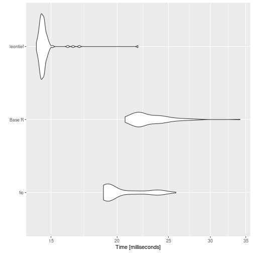
{fio} again faster.
Field of influence
Since field of influence involves computing Leontief inverse matrix for each element of technical coefficients matrix after an increment, it can be demanding for high dimensional matrices. Here, we evaluate benchmark for base R function and {fio}, since there’s no similiar function in {leontief}. For brevity, we cut dimensions to 100 and repetitions to 10.
# base R function
field_influence_r <- function(A, B, ee = 0.001) {
  n = nrow(A)
  I = diag(n)
  E = matrix(0, ncol = n, nrow = n)
  SI = matrix(0, ncol = n, nrow = n)
  for (i in 1:n) {
    for (j in 1:n) {
      E[i, j] = ee
      AE = A + E
      BE = solve(I - AE)
      FE = (BE - B) / ee
      FEq = FE * FE
      S = sum(FEq)
      SI[i, j] = S
      E[i, j] = 0
    }
  }
  return(SI) # Added return statement
}

# benchmark
benchmark_d <- bench::press(
  matrix_dim = c(30, 60, 100),
  {
    intermediate_transactions <- matrix(
      as.double(sample(1:1000, matrix_dim^2, replace = TRUE)),
      nrow = matrix_dim,
      ncol = matrix_dim
    )
    total_production <- matrix(
      as.double(sample(4000000:6000000, matrix_dim, replace = TRUE)),
      nrow = 1,
      ncol = matrix_dim
    )
    iom_fio_reduced <- fio::iom$new(
      "iom_reduced",
      intermediate_transactions,
      total_production
    )$compute_tech_coeff()$compute_leontief_inverse()
    bench::mark(
      fio = fio:::compute_field_influence(
        iom_fio_reduced$technical_coefficients_matrix,
        iom_fio_reduced$leontief_inverse_matrix,
        0.001
      ),
      `Base R` = field_influence_r(
        iom_fio_reduced$technical_coefficients_matrix,
        iom_fio_reduced$leontief_inverse_matrix
      ),
      iterations = 10,
      check = FALSE
    )
  }
)
#> Running with:
#>   matrix_dim
#> 1         30
#> 2         60
#> Warning: Some expressions had a GC in every iteration; so filtering is
#> disabled.
#> 3        100
#> Warning: Some expressions had a GC in every iteration; so filtering is
#> disabled.
print(benchmark_d)
#> # A tibble: 6 × 14
#>   expression matrix_dim      min   median `itr/sec` mem_alloc `gc/sec` n_itr
#>   <bch:expr>      <dbl> <bch:tm> <bch:tm>     <dbl> <bch:byt>    <dbl> <int>
#> 1 fio                30   5.47ms   5.51ms   181.      16.67KB     0       10
#> 2 Base R             30  23.76ms  24.17ms    41.3     44.52MB    10.3      8
#> 3 fio                60 111.41ms 111.72ms     8.95    56.34KB     0       10
#> 4 Base R             60 718.27ms 726.39ms     1.37    701.2MB     2.75    10
#> 5 fio               100     3.6s    5.07s     0.203  156.34KB     0       10
#> 6 Base R            100    4.24s    4.26s     0.234    5.25GB     3.83    10
#> # ℹ 6 more variables: n_gc <dbl>, total_time <bch:tm>, result <list>,
#> #   memory <list>, time <list>, gc <list>
ggplot2::autoplot(benchmark_d)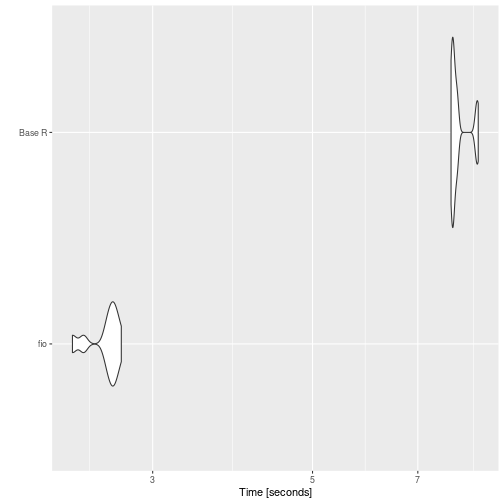
{fio} faster.
Or in a equivalent way, multiplying intermediate transactions matrix by a diagonal matrix constructed from total production vector.↩︎