DISCLAIMER
The present benchmark was conducted on 2025-06-17 on a Intel® Core™
i5-7400 (4-core CPU, AMD Radeon™ RX 580 2048SP GPU, 16GB RAM, Ubuntu
24.04). Results will vary depending on the hardware. These
benchmarks aim to provide a general idea of the performance differences
between the fio package and other implementations but
should not be considered definitive. The performance of the functions
may also vary depending on the specific data used and the context in
which they are applied.
Introduction
This vignette presents a benchmarking analysis comparing the
performance of functions from the fio package with
equivalent base R functions and functions from other packages. The
fio package provides a set of functions for input-output
analysis, a method used in economics to analyze the interdependencies
between different sectors of an economy.
Our benchmarking tests show that fio package functions
are generally faster than other implementations. This improved
performance can make a substantial difference in larger analyses, making
the fio package a valuable tool for input-output analysis
in R.
The tests were run on simulated square matrices, with dimensions ranging from 100x100 up to 2000x2000, and each test was repeated at least 10 times to account for variability. Please note that the results of this benchmarking analysis depend on the specific test datasets used and the hardware on which the algorithms were run. Therefore, the results should be interpreted in the context of these specific conditions.
Technical coefficients matrix
The technical coefficients matrix calculation, a key and initial step
in input-output analysis, was tested using the
compute_tech_coeff() function from the fio
package, equivalent functions from the leontief package,
and a base R implementation. It consists of dividing each
element of the intermediate transactions matrix by the corresponding
element of the total production vector1.
Results shows that {fio} is generally faster than the other two implementations, especially for larger matrices (≥500x500).
# set seed
set.seed(100)

# Base R function
tech_coeff_r <- function(intermediate_transactions, total_production) {
  tech_coeff_matrix <- intermediate_transactions %*% diag(1 / as.vector(total_production))
  return(tech_coeff_matrix)
}

# benchmark
benchmark_a <- bench::press(
  matrix_dim = c(100, 500, 1000, 2000),
  {
    intermediate_transactions <- matrix(
      as.double(sample(1:1000, matrix_dim^2, replace = TRUE)),
      nrow = matrix_dim,
      ncol = matrix_dim
    )
    total_production <- matrix(
      as.double(sample(4000000:6000000, matrix_dim, replace = TRUE)),
      nrow = 1,
      ncol = matrix_dim
    )
    iom_fio <- fio::iom$new("iom", intermediate_transactions, total_production)
    bench::mark(
      fio = fio:::compute_tech_coeff(intermediate_transactions, total_production),
      `Base R` = tech_coeff_r(intermediate_transactions, total_production),
      leontief = leontief::input_requirement(intermediate_transactions, total_production),
      iterations = 100
    )
  }
)
#> Running with:
#>   matrix_dim
#> 1        100
#> 2        500
#> 3       1000
#> 4       2000
#> Warning: Some expressions had a GC in every iteration; so filtering is disabled.
print(benchmark_a)
#> # A tibble: 12 × 9
#>    expression matrix_dim      min   median mem_alloc  `gc/sec` n_itr  n_gc total_time
#>    <bch:expr>      <dbl> <bch:tm> <bch:tm> <bch:byt>     <dbl> <int> <dbl>   <bch:tm>
#>  1 fio               100 108.97µs 148.26µs  861.82KB    0        100     0     15.4ms
#>  2 Base R            100 722.76µs 730.42µs  190.67KB    0        100     0    77.31ms
#>  3 leontief          100 311.21µs 325.95µs  724.27KB   23.8       99     1    41.95ms
#>  4 fio               500   1.22ms   2.16ms    1.91MB   23.6       95     5   211.83ms
#>  5 Base R            500  75.66ms   79.4ms    3.82MB    1.38      90    10      7.25s
#>  6 leontief          500   4.37ms   4.63ms   16.29MB  354.        39    66   186.45ms
#>  7 fio              1000   7.65ms   7.81ms    7.63MB   19.0       87    13   685.64ms
#>  8 Base R           1000  718.2ms 726.26ms   15.27MB    0.708     66    34        48s
#>  9 leontief         1000  35.74ms  35.84ms      65MB 2121.         2   152    71.68ms
#> 10 fio              2000  18.03ms  29.62ms   30.52MB    5.39     100    16      2.97s
#> 11 Base R           2000    6.01s    6.04s   61.05MB    0.0613   100    37     10.06m
#> 12 leontief         2000  71.69ms 125.73ms   259.7MB   21.6      100   272     12.58s

# plot
ggplot2::autoplot(benchmark_a)
For larger matrices (≥500x500), {fio} is generally faster.
Leontief inverse matrix
The Leontief matrix () is obtained by subtracting the technical coefficients matrix () from the identity matrix (); therefore, it has no null rows or columns. This allows for solving the linear system through LU decomposition, which is a more efficient method than direct inverse matrix calculation.
Results shows that {fio} is substantially faster.
# base R function
leontief_inverse_r <- function(technical_coefficients_matrix) {
  dim <- nrow(technical_coefficients_matrix)
  leontief_inverse_matrix <- solve(diag(dim) - technical_coefficients_matrix)
  return(leontief_inverse_matrix)
}

# benchmark
benchmark_b <- bench::press(
  matrix_dim = c(100, 500, 1000, 2000),
  {
    intermediate_transactions <- matrix(
      as.double(sample(1:1000, matrix_dim^2, replace = TRUE)),
      nrow = matrix_dim,
      ncol = matrix_dim
    )
    total_production <- matrix(
      as.double(sample(4000000:6000000, matrix_dim, replace = TRUE)),
      nrow = 1,
      ncol = matrix_dim
    )
    iom_fio <- fio::iom$new("iom", intermediate_transactions, total_production)
    iom_fio$compute_tech_coeff()
    technical_coefficients_matrix <- iom_fio$technical_coefficients_matrix
    bench::mark(
      fio = fio:::compute_leontief_inverse(technical_coefficients_matrix),
      `Base R` = leontief_inverse_r(technical_coefficients_matrix),
      leontief = leontief::leontief_inverse(technical_coefficients_matrix),
      iterations = 100,
      check = FALSE
    )
  }
)
#> Running with:
#>   matrix_dim
#> 1        100
#> 2        500
#> 3       1000
#> 4       2000
print(benchmark_b)
#> # A tibble: 12 × 9
#>    expression matrix_dim      min   median mem_alloc `gc/sec` n_itr  n_gc total_time
#>    <bch:expr>      <dbl> <bch:tm> <bch:tm> <bch:byt>    <dbl> <int> <dbl>   <bch:tm>
#>  1 fio               100 476.68µs 492.41µs  158.51KB    0       100     0    56.45ms
#>  2 Base R            100 834.58µs 843.59µs  413.29KB    0       100     0    87.94ms
#>  3 leontief          100 837.19µs 846.39µs  402.57KB    0       100     0    85.19ms
#>  4 fio               500   8.57ms   9.93ms    3.81MB    0.925    99     1      1.08s
#>  5 Base R            500  82.82ms  83.51ms    9.55MB    1.03     92     8      7.74s
#>  6 leontief          500  82.91ms  83.29ms    9.55MB    1.18     91     9       7.6s
#>  7 fio              1000  41.35ms  43.24ms   15.26MB    1.69     93     7      4.14s
#>  8 Base R           1000 669.08ms 681.85ms   38.18MB    0.389    79    21     53.94s
#>  9 leontief         1000  672.2ms 682.89ms   38.18MB    0.412    78    22     53.43s
#> 10 fio              2000 236.29ms 247.58ms   61.03MB    1.04     79    21     20.21s
#> 11 Base R           2000     6.4s    6.41s  152.66MB    0.467    26    78      2.78m
#> 12 leontief         2000    6.39s     6.4s  152.66MB    0.156    50    50      5.34m

# plot
ggplot2::autoplot(benchmark_b)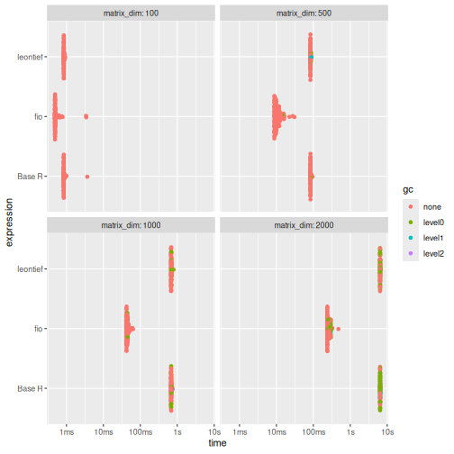
{fio} is substantially faster.
Sensitivity of dispersion coefficients of variation
To evaluate the performance of linkage-based functions, we benchmarked the sensitivity of dispersion coefficients of variation.
Results shows that {fio} is substantially faster than {leontief} across all tested dimensions. Compared to Base R, {fio} is faster for matrices 500x500 and larger.
# base R function
sensitivity_r <- function(B) {
  n <- nrow(B)
  SL = rowSums(B)
  ML = SL / n
  (((1 / (n - 1)) * (colSums((B - ML) ** 2))) ** 0.5) / ML
}

# benchmark
benchmark_c <- bench::press(
  matrix_dim = c(100, 500, 1000, 2000),
  {
    intermediate_transactions <- matrix(
      as.double(sample(1:1000, matrix_dim^2, replace = TRUE)),
      nrow = matrix_dim,
      ncol = matrix_dim
    )
    total_production <- matrix(
      as.double(sample(4000000:6000000, matrix_dim, replace = TRUE)),
      nrow = 1,
      ncol = matrix_dim
    )
    iom_fio <- fio::iom$new("iom", intermediate_transactions, total_production)
    iom_fio$compute_tech_coeff()$compute_leontief_inverse()
    leontief_inverse_matrix <- iom_fio$leontief_inverse_matrix
    bench::mark(
      fio = fio:::compute_sensitivity_dispersion_cv(leontief_inverse_matrix),
      `Base R` = sensitivity_r(leontief_inverse_matrix),
      leontief = leontief::sensitivity_dispersion_cv(leontief_inverse_matrix),
      iterations = 100,
      check = FALSE
    )
  }
)
#> Running with:
#>   matrix_dim
#> 1        100
#> 2        500
#> 3       1000
#> 4       2000
#> Warning: Some expressions had a GC in every iteration; so filtering is disabled.
print(benchmark_c)
#> # A tibble: 12 × 9
#>    expression matrix_dim      min   median mem_alloc `gc/sec` n_itr  n_gc total_time
#>    <bch:expr>      <dbl> <bch:tm> <bch:tm> <bch:byt>    <dbl> <int> <dbl>   <bch:tm>
#>  1 fio               100  104.9µs 117.43µs   81.23KB     0      100     0    13.13ms
#>  2 Base R            100  59.04µs  59.95µs   81.48KB     0      100     0    14.05ms
#>  3 leontief          100   1.39ms   1.42ms  745.38KB     6.74    99     1   148.37ms
#>  4 fio               500 695.04µs 797.88µs    1.91MB     0      100     0    79.91ms
#>  5 Base R            500   1.14ms   1.95ms    1.92MB     0      100     0      181ms
#>  6 leontief          500  27.78ms  28.01ms   17.31MB     2.66    93     7      2.63s
#>  7 fio              1000   3.11ms    3.3ms    7.64MB     0      100     0   335.86ms
#>  8 Base R           1000   4.82ms   4.87ms    7.66MB     8.37    96     4   477.94ms
#>  9 leontief         1000 155.33ms 156.15ms   68.94MB     3.29    66    34     10.33s
#> 10 fio              2000  14.83ms  15.02ms   30.53MB     0      100     0      1.52s
#> 11 Base R           2000  19.37ms  32.08ms   30.58MB     4.23   100    12      2.84s
#> 12 leontief         2000 744.88ms 822.07ms  275.22MB     3.35   100   276      1.37m

# plot
ggplot2::autoplot(benchmark_c)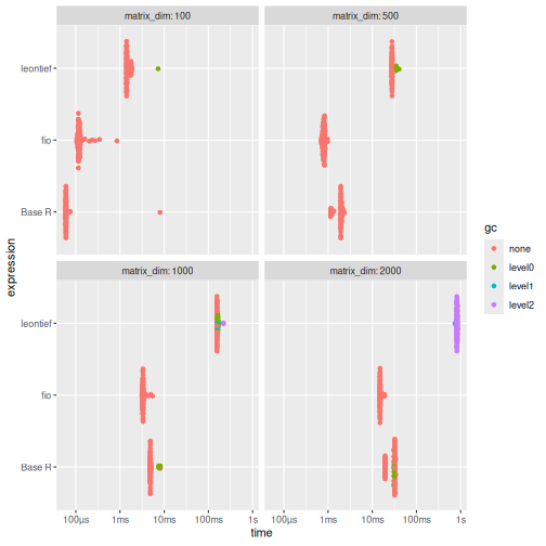
{fio} is substantially faster than {leontief} across all tested dimensions. Compared to Base R, {fio} is faster for matrices 500x500 and larger.
Field of influence
Since computing the field of influence involves calculating the Leontief inverse matrix for each element of the technical coefficients matrix after an increment, it can be demanding for high-dimensional matrices. Here, we benchmark the base R function and fio, as there is no similar function in leontief. For brevity, we limited the matrix dimensions to 100x100 and the number of repetitions to 10.
Results shows that {fio} is almost two times faster than the base R implementation.
# base R function
field_influence_r <- function(A, B, ee = 0.001) {
  n = nrow(A)
  I = diag(n)
  E = matrix(0, ncol = n, nrow = n)
  SI = matrix(0, ncol = n, nrow = n)
  for (i in 1:n) {
    for (j in 1:n) {
      E[i, j] = ee
      AE = A + E
      BE = solve(I - AE)
      FE = (BE - B) / ee
      FEq = FE * FE
      S = sum(FEq)
      SI[i, j] = S
      E[i, j] = 0
    }
  }
  return(SI) # Added return statement
}

# benchmark
benchmark_d <- bench::press(
  matrix_dim = c(30, 60, 100),
  {
    intermediate_transactions <- matrix(
      as.double(sample(1:1000, matrix_dim^2, replace = TRUE)),
      nrow = matrix_dim,
      ncol = matrix_dim
    )
    total_production <- matrix(
      as.double(sample(4000000:6000000, matrix_dim, replace = TRUE)),
      nrow = 1,
      ncol = matrix_dim
    )
    iom_fio_reduced <- fio::iom$new(
      "iom_reduced",
      intermediate_transactions,
      total_production
    )$compute_tech_coeff()$compute_leontief_inverse()
    bench::mark(
      fio = fio:::compute_field_influence(
        iom_fio_reduced$technical_coefficients_matrix,
        iom_fio_reduced$leontief_inverse_matrix,
        0.001
      ),
      `Base R` = field_influence_r(
        iom_fio_reduced$technical_coefficients_matrix,
        iom_fio_reduced$leontief_inverse_matrix
      ),
      iterations = 10,
      check = FALSE
    )
  }
)
#> Running with:
#>   matrix_dim
#> 1         30
#> 2         60
#> Warning: Some expressions had a GC in every iteration; so filtering is disabled.
#> 3        100
#> Warning: Some expressions had a GC in every iteration; so filtering is disabled.
print(benchmark_d)
#> # A tibble: 6 × 9
#>   expression matrix_dim      min   median mem_alloc `gc/sec` n_itr  n_gc total_time
#>   <bch:expr>      <dbl> <bch:tm> <bch:tm> <bch:byt>    <dbl> <int> <dbl>   <bch:tm>
#> 1 fio                30   49.3ms  49.59ms  16.66KB     0       10     0   496.66ms
#> 2 Base R             30  53.92ms  54.84ms  44.52MB     4.56     8     2   438.77ms
#> 3 fio                60 802.29ms 809.86ms  56.34KB     0       10     0      8.26s
#> 4 Base R             60 890.07ms  893.2ms  701.2MB     2.23    10    20      8.98s
#> 5 fio               100    4.64s    4.71s 156.34KB     0       10     0     47.72s
#> 6 Base R            100    8.93s    8.95s   5.25GB     1.95    10   175       1.5m
ggplot2::autoplot(benchmark_d)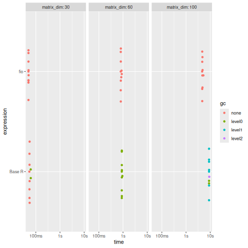
Across all matrix sizes, {fio} demonstrates superior performance, being considerably faster than the Base R implementation.