Multi-Regional Input-Output Analysis

Introduction

Multi-Regional Input-Output (MRIO) analysis extends traditional input-output analysis to capture economic interdependencies between multiple regions or countries. The miom class in the fio package implements the methodology described in Miller & Blair (2009) for analyzing multi-regional economic systems.

This vignette demonstrates how to:

Create and work with multi-regional input-output matrices
Compute multi-regional multipliers
Analyze inter-regional spillover effects
Extract country-specific input-output tables
Measure regional interdependence

In a multi-regional system with $R$ regions and $N$ sectors per region, the total dimensions of the system are $RN \times RN$ . The intermediate transactions matrix $\mathbf{Z}$ is partitioned as:

$\mathbf{Z} = \begin{bmatrix} \mathbf{Z}^{11} & \mathbf{Z}^{12} & \cdots & \mathbf{Z}^{1R} \\ \mathbf{Z}^{21} & \mathbf{Z}^{22} & \cdots & \mathbf{Z}^{2R} \\ \vdots & \vdots & \ddots & \vdots \\ \mathbf{Z}^{R1} & \mathbf{Z}^{R2} & \cdots & \mathbf{Z}^{RR} \end{bmatrix}$

where $\mathbf{Z}^{rs}$ represents intermediate flows from region $s$ to region $r$ .

Computations of the multi-regional Leontief inverse is the same from the single-region case:

$\mathbf{L} = (\mathbf{I} - \mathbf{A})^{-1}$

where $\mathbf{A}$ is the multi-regional technical coefficients matrix. Therefore, the multi-regional input-output class miom is able to inherit methods from the iom class, implementing the additional functionality needed for multi-regional analysis.

SHOWCASING THE `miom` CLASS: 2000 WORLD ECONOMY EXAMPLE

The fiodata package includes the world_2000 dataset, which contains real multi-regional input-output data for 26 countries and 23 sectors from the year 2000. This dataset was created using element-by-element imports from Excel files with import_element() as demonstrated in the World 2000 script.

Let’s load and examine this real-world dataset:

# import real-world dataset
world_2000 <- fiodata::world_2000

# Examine the structure
world_2000$n_countries
#> [1] 26
world_2000$n_sectors
#> [1] 23
nrow(world_2000$intermediate_transactions)
#> [1] 598
ncol(world_2000$intermediate_transactions)
#> [1] 598

# Show the countries and sectors
world_2000$countries
#>  [1] "AUS" "AUT" "BEL" "BRA" "CAN" "CHN" "DEU" "DNK" "ESP" "FIN" "FRA" "GBR"
#> [13] "GRC" "HKG" "IND" "IRL" "ITA" "JPN" "KOR" "MEX" "NDL" "PRT" "SWE" "TWN"
#> [25] "USA" "ROW"
world_2000$sectors
#>  [1] "Agriculture, Hunting, Forestry and Fishing" 
#>  [2] "Mining and Quarrying"                       
#>  [3] "Food, Beverages and Tobacco"                
#>  [4] "Textiles, leather and footwear"             
#>  [5] "Pulp, paper, printing and publishing"       
#>  [6] "Coke, refined petroleum and nuclear fuel"   
#>  [7] "Chemicals and chemicals products"           
#>  [8] "Rubber and plastics"                        
#>  [9] "Other non-metallic mineral"                 
#> [10] "Basic metals and fabricated metal"          
#> [11] "Machinery"                                  
#> [12] "Electrical and optical equipment"           
#> [13] "Transport equipment"                        
#> [14] "Manufacturing, recycling"                   
#> [15] "Electricity, gas and water supply"          
#> [16] "Construction"                               
#> [17] "Wholesale and retail trade"                 
#> [18] "Hotels and restaurants"                     
#> [19] "Transport and storage"                      
#> [20] "Post and telecommunications"                
#> [21] "Financial intermediation"                   
#> [22] "Real state, renting and business activities"
#> [23] "Community, social and personal services"

# Show a small subset of transactions (first 6 countries x sectors)
knitr::kable(
  world_2000$intermediate_transactions[1:6, 1:6],
  digits = 0,
  caption = "Sample of Intermediate Transactions (millions of dollars)"
)

Sample of Intermediate Transactions (millions of dollars)
	AUS_Agriculture, Hunting, Forestry and Fishing	AUS_Mining and Quarrying	AUS_Food, Beverages and Tobacco	AUS_Textiles, leather and footwear	AUS_Pulp, paper, printing and publishing	AUS_Coke, refined petroleum and nuclear fuel
AUS_Agriculture, Hunting, Forestry and Fishing	2976	16	8128	538	163	0
AUS_Mining and Quarrying	17	1881	117	11	34	3355
AUS_Food, Beverages and Tobacco	796	33	3387	68	21	14
AUS_Textiles, leather and footwear	25	15	54	565	29	6
AUS_Pulp, paper, printing and publishing	92	75	834	56	2193	15
AUS_Coke, refined petroleum and nuclear fuel	359	452	61	6	41	331


# Show total production for first few country-sectors
knitr::kable(
  t(world_2000$total_production[1, 1:6]),
  digits = 0,
  caption = "Sample of Total Production (millions of dollars)"
)

Sample of Total Production (millions of dollars)
AUS_Agriculture, Hunting, Forestry and Fishing	AUS_Mining and Quarrying	AUS_Food, Beverages and Tobacco	AUS_Textiles, leather and footwear	AUS_Pulp, paper, printing and publishing	AUS_Coke, refined petroleum and nuclear fuel
28170	35785	35716	5857	15198	9871

The intermediate transactions matrix shows the flows of goods and services between all country-sector combinations in the global economy. The values represent monetary flows in millions of dollars. Each element represents purchases of intermediate inputs from the supplying country-sector (columns) by the purchasing country-sector (rows). It captures the complete structure of intermediate transactions between 26 countries across 23 economic sectors, providing a comprehensive view of global economic interdependencies in the year 2000.

Multi-Regional Multiplier Analysis

The miom class computes several types of multipliers following Miller & Blair (2009):

Intra-regional multipliers: Effects within the same region
Spillover multipliers: Effects on other regions
Total multipliers: Sum of intra-regional and spillover effects

world_2000$compute_multiregional_multipliers()

# Show first 10 rows of multipliers for readability
knitr::kable(
  world_2000$multiregional_multipliers[1:10, 1:10],
  digits = 4,
  caption = "Multi-Regional Multipliers (first 10 country-sectors)"
)

Multi-Regional Multipliers (first 10 country-sectors)
shock_country	shock_sector	shock_label	intra_regional_multiplier	spillover_multiplier	total_multiplier	multiplier_to_AUS	multiplier_to_AUT	multiplier_to_BEL	multiplier_to_BRA
AUS	Agriculture, Hunting, Forestry and Fishing	AUS_Agriculture, Hunting, Forestry and Fishing	1.8179	0.2331	2.0510	1.8179	0.0012	0.0031	0.0019
AUS	Mining and Quarrying	AUS_Mining and Quarrying	1.6935	0.2127	1.9061	1.6935	0.0011	0.0020	0.0012
AUS	Food, Beverages and Tobacco	AUS_Food, Beverages and Tobacco	2.3286	0.2703	2.5990	2.3286	0.0015	0.0030	0.0027
AUS	Textiles, leather and footwear	AUS_Textiles, leather and footwear	2.0626	0.4556	2.5181	2.0626	0.0025	0.0056	0.0029
AUS	Pulp, paper, printing and publishing	AUS_Pulp, paper, printing and publishing	2.0275	0.3072	2.3347	2.0275	0.0022	0.0039	0.0024
AUS	Coke, refined petroleum and nuclear fuel	AUS_Coke, refined petroleum and nuclear fuel	2.2922	0.4806	2.7728	2.2922	0.0018	0.0036	0.0021
AUS	Chemicals and chemicals products	AUS_Chemicals and chemicals products	2.1035	0.5020	2.6055	2.1035	0.0024	0.0079	0.0035
AUS	Rubber and plastics	AUS_Rubber and plastics	1.9421	0.4697	2.4118	1.9421	0.0023	0.0074	0.0031
AUS	Other non-metallic mineral	AUS_Other non-metallic mineral	2.0107	0.3092	2.3199	2.0107	0.0017	0.0031	0.0022
AUS	Basic metals and fabricated metal	AUS_Basic metals and fabricated metal	2.0796	0.3984	2.4779	2.0796	0.0022	0.0034	0.0023

Interpreting the Multipliers

The multipliers table shows several key measures for each country-sector combination (each row is a $1 final-demand shock in shock_country / shock_sector):

Intra-regional multiplier: The total effect within the same country when that sector receives a $1 shock
Spillover multiplier: The total effect on all other countries from the same shock
Total multiplier: The sum of intra-regional and spillover effects
Multiplier to [Country]: The specific spillover effect on each individual country

Let’s find an interesting example. Take a look at Brazil Agriculture and it’s effects on USA:

# Find Brazil agriculture row
bra_agr_index <- which(grepl("BRA.*Agriculture", world_2000$multiregional_multipliers$shock_label))[1]
bra_agr <- world_2000$multiregional_multipliers[bra_agr_index, ]

# Show key multiplier components
multiplier_cols <- c("shock_label", "intra_regional_multiplier", "spillover_multiplier", "total_multiplier", "multiplier_to_USA")
available_cols <- intersect(multiplier_cols, names(bra_agr))
knitr::kable(bra_agr[, available_cols],
  digits = 4,
  caption = "Example: Brazil Agriculture Multipliers"
)

Example: Brazil Agriculture Multipliers
	shock_label	intra_regional_multiplier	spillover_multiplier	total_multiplier	multiplier_to_USA
70	BRA_Agriculture, Hunting, Forestry and Fishing	1.6809	0.1691	1.85	0.0385

The multipliers reveal important insights about global economic linkages. The intra-regional multiplier shows the domestic effect within a country when one of its sectors receives a demand shock, while the spillover multiplier captures the total impact on all other countries.

Spillover Matrix

The spillover matrix provides a comprehensive view of how shocks in each country-sector affect all other country-sectors in the system:

spillover_matrix <- world_2000$get_spillover_matrix()

This $598 \times 598$ matrix contains the complete set of multiplier effects. For example, we can examine how a shock to the US electrical sector affects manufacturing in other countries:

# Effects of a shock to US Electrical sector
electrical_effects <- spillover_matrix[grepl("Manufacturing", rownames(spillover_matrix)), "USA_Electrical and optical equipment"]
knitr::kable(
  electrical_effects,
  digits = 10,
  caption = "Effects of a unit shock to US Electrical sector"
)

Effects of a unit shock to US Electrical sector
	x
AUS_Manufacturing, recycling	0.0000278285
AUT_Manufacturing, recycling	0.0000317729
BEL_Manufacturing, recycling	0.0000746418
BRA_Manufacturing, recycling	0.0000750513
CAN_Manufacturing, recycling	0.0010488480
CHN_Manufacturing, recycling	0.0005086378
DEU_Manufacturing, recycling	0.0001300296
DNK_Manufacturing, recycling	0.0000092364
ESP_Manufacturing, recycling	0.0000666478
FIN_Manufacturing, recycling	0.0000274000
FRA_Manufacturing, recycling	0.0001874089
GBR_Manufacturing, recycling	0.0001376910
GRC_Manufacturing, recycling	0.0000050262
HKG_Manufacturing, recycling	0.0000204918
IND_Manufacturing, recycling	0.0001132960
IRL_Manufacturing, recycling	0.0000133946
ITA_Manufacturing, recycling	0.0001741727
JPN_Manufacturing, recycling	0.0002515836
KOR_Manufacturing, recycling	0.0000513328
MEX_Manufacturing, recycling	0.0003234464
NDL_Manufacturing, recycling	0.0000272870
PRT_Manufacturing, recycling	0.0000232974
SWE_Manufacturing, recycling	0.0000563693
TWN_Manufacturing, recycling	0.0001025605
USA_Manufacturing, recycling	0.0000000000
ROW_Manufacturing, recycling	0.0009231601

These values show the output response in each foreign country-sector to a unit shock in USA Electrical and optical equipment.

Net Spillover Effects

Net spillover effects reveal asymmetric cross-regional multiplier linkages. For countries $r$ and $s$ , $net[r, s] = spillover_{s→r} - spillover_{r→s}$ (block sums from the spillover matrix).

net_spillover <- world_2000$get_net_spillover_matrix()
knitr::kable(net_spillover, digits = 4, caption = "Net Spillover Effects Matrix")

Net Spillover Effects Matrix
	AUS	AUT	BEL	BRA	CAN	CHN	DEU	DNK	ESP	FIN	FRA	GBR	GRC	HKG	IND	IRL	ITA	JPN	KOR	MEX	NDL	PRT	SWE	TWN	USA	ROW
AUS	0.0000	-0.0128	0.0161	0.0185	-0.0666	-0.2094	-0.3254	0.0054	-0.0169	0.1028	-0.1678	-0.3081	0.0373	0.2802	0.1332	0.0170	-0.1683	-0.4861	0.2846	-0.0004	0.0029	0.0107	-0.0414	0.6035	-1.4584	-1.6443
AUT	0.0128	0.0000	-0.1123	-0.0255	-0.0542	-0.1683	-3.4544	0.0801	-0.1197	0.0000	-0.5047	-0.3707	0.1085	0.0251	-0.0127	0.0583	-0.7356	-0.3207	-0.0394	-0.0077	-0.2614	0.0610	-0.0481	-0.0705	-0.8216	-2.0690
BEL	-0.0161	0.1123	0.0000	-0.1303	-0.1564	-0.2612	-2.1978	0.3258	-0.1575	0.0651	-1.5795	-1.3692	0.2773	0.1062	0.0709	0.0739	-0.4425	-0.5333	-0.0801	-0.0204	-1.2560	0.2428	-0.0370	0.0316	-1.7541	-2.2477
BRA	-0.0185	0.0255	0.1303	0.0000	-0.0638	-0.1074	-0.3114	0.0543	-0.0272	0.0703	-0.1351	-0.1205	0.0703	0.1400	-0.0121	0.0602	-0.1189	-0.3053	-0.0575	0.0248	0.1271	0.1395	-0.0003	-0.0139	-1.1401	-1.3336
CAN	0.0666	0.0542	0.1564	0.0638	0.0000	-0.1215	-0.1589	0.0738	-0.0062	0.0598	-0.0793	-0.3592	0.0755	0.4725	0.0422	0.2618	-0.0790	-0.3763	0.0299	0.0400	0.0914	0.0575	0.0410	-0.0074	-4.7295	-0.9500
CHN	0.2094	0.1683	0.2612	0.1074	0.1215	0.0000	-0.0647	0.2008	0.1432	0.1481	0.0488	0.0196	0.1972	3.2840	0.1929	0.2366	0.0578	-0.9235	0.0400	0.1713	0.2811	0.1269	0.0763	-0.1745	-0.4623	-1.0555
DEU	0.3254	3.4544	2.1978	0.3114	0.1589	0.0647	0.0000	2.0943	0.9054	1.1904	0.4801	0.1591	1.2163	0.6132	0.2229	0.9037	0.4094	-0.2973	0.1949	0.2775	1.4774	1.4083	1.6150	0.8653	-0.7504	-1.2917
DNK	-0.0054	-0.0801	-0.3258	-0.0543	-0.0738	-0.2008	-2.0943	0.0000	-0.1529	-0.0126	-0.6395	-1.0682	0.0649	0.0549	-0.0269	0.0893	-0.5411	-0.2305	-0.0836	-0.0077	-0.5998	0.0259	-0.8529	-0.0162	-0.7998	-1.9055
ESP	0.0169	0.1197	0.1575	0.0272	0.0062	-0.1432	-0.9054	0.1529	0.0000	0.0762	-0.8883	-0.4055	0.3551	0.1613	-0.0049	0.2886	-0.6444	-0.2458	-0.0200	-0.0514	0.0455	2.4591	0.0988	0.1080	-0.5864	-1.8137
FIN	-0.1028	0.0000	-0.0651	-0.0703	-0.0598	-0.1481	-1.1904	0.0126	-0.0762	0.0000	-0.4082	-0.5926	0.1242	0.0389	-0.0104	0.0738	-0.3406	-0.4668	-0.0713	-0.0079	-0.2015	0.0461	-0.3288	-0.0692	-0.9072	-2.3061
FRA	0.1678	0.5047	1.5795	0.1351	0.0793	-0.0488	-0.4801	0.6395	0.8883	0.4082	0.0000	-0.1323	0.7620	0.4191	0.1152	0.8238	0.0105	-0.2843	0.1093	0.0987	0.6057	1.0754	0.7666	0.1600	-0.8321	-1.2457
GBR	0.3081	0.3707	1.3692	0.1205	0.3592	-0.0196	-0.1591	1.0682	0.4055	0.5926	0.1323	0.0000	0.5151	0.5883	0.3410	4.1994	0.0674	-0.3685	0.0660	0.0746	1.0018	0.7635	1.0191	0.5895	-1.0395	-1.1629
GRC	-0.0373	-0.1085	-0.2773	-0.0703	-0.0755	-0.1972	-1.2163	-0.0649	-0.3551	-0.1242	-0.7620	-0.5151	0.0000	-0.0519	-0.0550	-0.0608	-1.6529	-0.2026	-0.1080	-0.0129	-0.4536	-0.0221	-0.2269	-0.0965	-0.5765	-3.1367
HKG	-0.2802	-0.0251	-0.1062	-0.1400	-0.4725	-3.2840	-0.6132	-0.0549	-0.1613	-0.0389	-0.4191	-0.5883	0.0519	0.0000	0.0359	0.1734	-0.6494	-2.3815	-1.3598	-0.0428	-0.3130	0.0171	-0.0231	-0.4679	-3.2704	-6.2372
IND	-0.1332	0.0127	-0.0709	0.0121	-0.0422	-0.1929	-0.2229	0.0269	0.0049	0.0104	-0.1152	-0.3410	0.0550	-0.0359	0.0000	0.0811	-0.0916	-0.3318	-0.0870	0.0157	-0.0116	0.0606	-0.0037	-0.0025	-0.5878	-2.9286
IRL	-0.0170	-0.0583	-0.0739	-0.0602	-0.2618	-0.2366	-0.9037	-0.0893	-0.2886	-0.0738	-0.8238	-4.1994	0.0608	-0.1734	-0.0811	0.0000	-0.5089	-0.6792	-0.2360	-0.0227	-0.3643	0.0139	-0.1881	-0.1746	-3.0383	-2.1441
ITA	0.1683	0.7356	0.4425	0.1189	0.0790	-0.0578	-0.4094	0.5411	0.6444	0.3406	-0.0105	-0.0674	1.6529	0.6494	0.0916	0.5089	0.0000	-0.1670	0.0946	0.1297	0.1910	0.7478	0.3421	0.1276	-0.4831	-1.6802
JPN	0.4861	0.3207	0.5333	0.3053	0.3763	0.9235	0.2973	0.2305	0.2458	0.4668	0.2843	0.3685	0.2026	2.3815	0.3318	0.6792	0.1670	0.0000	1.5110	0.4463	0.5557	0.3128	0.3421	1.7225	-0.0264	-0.4335
KOR	-0.2846	0.0394	0.0801	0.0575	-0.0299	-0.0400	-0.1949	0.0836	0.0200	0.0713	-0.1093	-0.0660	0.1080	1.3598	0.0870	0.2360	-0.0946	-1.5110	0.0000	0.1797	0.0487	0.1268	0.0371	0.2292	-1.5061	-2.8225
MEX	0.0004	0.0077	0.0204	-0.0248	-0.0400	-0.1713	-0.2775	0.0077	0.0514	0.0079	-0.0987	-0.0746	0.0129	0.0428	-0.0157	0.0227	-0.1297	-0.4463	-0.1797	0.0000	0.0109	0.0932	-0.0369	-0.0638	-4.6417	-0.6929
NDL	-0.0029	0.2614	1.2560	-0.1271	-0.0914	-0.2811	-1.4774	0.5998	-0.0455	0.2015	-0.6057	-1.0018	0.4536	0.3130	0.0116	0.3643	-0.1910	-0.5557	-0.0487	-0.0109	0.0000	0.3416	0.1307	0.3147	-1.7635	-2.9057
PRT	-0.0107	-0.0610	-0.2428	-0.1395	-0.0575	-0.1269	-1.4083	-0.0259	-2.4591	-0.0461	-1.0754	-0.7635	0.0221	-0.0171	-0.0606	-0.0139	-0.7478	-0.3128	-0.1268	-0.0932	-0.3416	0.0000	-0.1161	-0.0513	-0.5927	-2.1151
SWE	0.0414	0.0481	0.0370	0.0003	-0.0410	-0.0763	-1.6150	0.8529	-0.0988	0.3288	-0.7666	-1.0191	0.2269	0.0231	0.0037	0.1881	-0.3421	-0.3421	-0.0371	0.0369	-0.1307	0.1161	0.0000	-0.0189	-0.9712	-1.8780
TWN	-0.6035	0.0705	-0.0316	0.0139	0.0074	0.1745	-0.8653	0.0162	-0.1080	0.0692	-0.1600	-0.5895	0.0965	0.4679	0.0025	0.1746	-0.1276	-1.7225	-0.2292	0.0638	-0.3147	0.0513	0.0189	0.0000	-1.2744	-2.5937
USA	1.4584	0.8216	1.7541	1.1401	4.7295	0.4623	0.7504	0.7998	0.5864	0.9072	0.8321	1.0395	0.5765	3.2704	0.5878	3.0383	0.4831	0.0264	1.5061	4.6417	1.7635	0.5927	0.9712	1.2744	0.0000	0.7676
ROW	1.6443	2.0690	2.2477	1.3336	0.9500	1.0555	1.2917	1.9055	1.8137	2.3061	1.2457	1.1629	3.1367	6.2372	2.9286	2.1441	1.6802	0.4335	2.8225	0.6929	2.9057	2.1151	1.8780	2.5937	-0.7676	0.0000

The interpretation is:

Positive net[r, s]: country r receives more cross-regional output response from shocks in s than s receives from shocks in r (row country is a net recipient relative to the column country).
Negative net[r, s]: the column country receives more than the row country.
Values close to zero: roughly symmetric spillover relationship.

For example, net["USA", "CHN"] > 0 means a unit final-demand shock in China induces more output response in the USA than a comparable shock in the USA induces in China.

Key Sectors Analysis

Key sectors analysis identifies sectors with strong backward and forward linkages in the multi-regional system:

world_2000$compute_key_sectors()

key_sectors_table <- world_2000$key_sectors[, c(
  "country", "sector_name",
  "power_dispersion", "sensitivity_dispersion", "key_sectors"
)]
knitr::kable(head(key_sectors_table), digits = 4, caption = "Key Sectors Analysis")

Key Sectors Analysis
country	sector_name	power_dispersion	sensitivity_dispersion	key_sectors
AUS	Agriculture, Hunting, Forestry and Fishing	0.9231	0.9372	Non-Key Sector
AUS	Mining and Quarrying	0.8579	1.3972	Strong Forward Linkage
AUS	Food, Beverages and Tobacco	1.1698	0.7489	Strong Backward Linkage
AUS	Textiles, leather and footwear	1.1334	0.5495	Strong Backward Linkage
AUS	Pulp, paper, printing and publishing	1.0508	0.7826	Strong Backward Linkage
AUS	Coke, refined petroleum and nuclear fuel	1.2480	0.6396	Strong Backward Linkage

Key sectors are defined as those with above-average values in both power dispersion (backward linkages) and sensitivity dispersion (forward linkages). If both values exceed 1, the sector is classified as a key sector.

knitr::kable(
  subset(key_sectors_table, key_sectors == "Key Sector"),
  digits = 4,
  caption = "World Key Sectors"
)

World Key Sectors
	country	sector_name	power_dispersion	sensitivity_dispersion	key_sectors
10	AUS	Basic metals and fabricated metal	1.1153	1.1820	Key Sector
19	AUS	Transport and storage	1.0424	1.3665	Key Sector
63	BEL	Wholesale and retail trade	1.0474	2.1698	Key Sector
65	BEL	Transport and storage	1.1411	1.5131	Key Sector
76	BRA	Chemicals and chemicals products	1.1417	1.2050	Key Sector
79	BRA	Basic metals and fabricated metal	1.0736	1.1132	Key Sector
119	CHN	Textiles, leather and footwear	1.3286	1.1093	Key Sector
120	CHN	Pulp, paper, printing and publishing	1.2516	1.0303	Key Sector
122	CHN	Chemicals and chemicals products	1.3459	1.9790	Key Sector
123	CHN	Rubber and plastics	1.4161	1.0886	Key Sector
125	CHN	Basic metals and fabricated metal	1.4585	2.4764	Key Sector
126	CHN	Machinery	1.3794	1.2067	Key Sector
127	CHN	Electrical and optical equipment	1.4747	1.6025	Key Sector
129	CHN	Manufacturing, recycling	1.2086	1.0453	Key Sector
130	CHN	Electricity, gas and water supply	1.2553	1.7450	Key Sector
132	CHN	Wholesale and retail trade	1.0484	2.1414	Key Sector
134	CHN	Transport and storage	1.0038	1.5373	Key Sector
145	DEU	Chemicals and chemicals products	1.0474	2.2578	Key Sector
146	DEU	Rubber and plastics	1.0202	1.0244	Key Sector
148	DEU	Basic metals and fabricated metal	1.0454	2.4121	Key Sector
149	DEU	Machinery	1.0253	1.3351	Key Sector
150	DEU	Electrical and optical equipment	1.0221	1.6899	Key Sector
151	DEU	Transport equipment	1.2205	1.5320	Key Sector
157	DEU	Transport and storage	1.0201	1.9335	Key Sector
180	DNK	Transport and storage	1.1129	1.1100	Key Sector
191	ESP	Chemicals and chemicals products	1.1491	1.1413	Key Sector
194	ESP	Basic metals and fabricated metal	1.1418	1.6170	Key Sector
203	ESP	Transport and storage	1.0117	1.4705	Key Sector
212	FIN	Pulp, paper, printing and publishing	1.0648	1.2643	Key Sector
217	FIN	Basic metals and fabricated metal	1.1967	1.1400	Key Sector
219	FIN	Electrical and optical equipment	1.1325	1.0286	Key Sector
235	FRA	Pulp, paper, printing and publishing	1.0948	1.0433	Key Sector
237	FRA	Chemicals and chemicals products	1.1763	1.4539	Key Sector
240	FRA	Basic metals and fabricated metal	1.0929	1.6608	Key Sector
242	FRA	Electrical and optical equipment	1.1437	1.1142	Key Sector
243	FRA	Transport equipment	1.3170	1.0230	Key Sector
260	GBR	Chemicals and chemicals products	1.0925	1.4232	Key Sector
263	GBR	Basic metals and fabricated metal	1.0614	1.4967	Key Sector
265	GBR	Electrical and optical equipment	1.1180	1.1481	Key Sector
268	GBR	Electricity, gas and water supply	1.1078	1.2209	Key Sector
269	GBR	Construction	1.0719	1.0766	Key Sector
274	GBR	Financial intermediation	1.0443	1.7971	Key Sector
302	HKG	Food, Beverages and Tobacco	1.1664	1.6876	Key Sector
328	IND	Coke, refined petroleum and nuclear fuel	1.0923	1.0242	Key Sector
329	IND	Chemicals and chemicals products	1.2440	1.2686	Key Sector
332	IND	Basic metals and fabricated metal	1.2139	1.4188	Key Sector
337	IND	Electricity, gas and water supply	1.0560	1.3664	Key Sector
341	IND	Transport and storage	1.0298	1.3372	Key Sector
364	IRL	Transport and storage	1.1478	1.0157	Key Sector
372	ITA	Textiles, leather and footwear	1.2000	1.0926	Key Sector
375	ITA	Chemicals and chemicals products	1.2347	1.2772	Key Sector
378	ITA	Basic metals and fabricated metal	1.1569	1.8881	Key Sector
379	ITA	Machinery	1.1753	1.0061	Key Sector
380	ITA	Electrical and optical equipment	1.1478	1.0112	Key Sector
383	ITA	Electricity, gas and water supply	1.0292	1.0177	Key Sector
387	ITA	Transport and storage	1.0400	1.7155	Key Sector
398	JPN	Chemicals and chemicals products	1.0680	2.0598	Key Sector
399	JPN	Rubber and plastics	1.0769	1.0362	Key Sector
401	JPN	Basic metals and fabricated metal	1.0922	2.2050	Key Sector
403	JPN	Electrical and optical equipment	1.0510	1.9391	Key Sector
404	JPN	Transport equipment	1.2852	1.3949	Key Sector
419	KOR	Pulp, paper, printing and publishing	1.2710	1.0932	Key Sector
420	KOR	Coke, refined petroleum and nuclear fuel	1.1157	1.2112	Key Sector
421	KOR	Chemicals and chemicals products	1.3239	1.8206	Key Sector
424	KOR	Basic metals and fabricated metal	1.3695	1.7999	Key Sector
426	KOR	Electrical and optical equipment	1.2945	1.3842	Key Sector
433	KOR	Transport and storage	1.0373	1.1349	Key Sector
467	NDL	Chemicals and chemicals products	1.1497	1.1829	Key Sector
498	PRT	Electricity, gas and water supply	1.0681	1.1445	Key Sector
511	SWE	Pulp, paper, printing and publishing	1.0473	1.0424	Key Sector
516	SWE	Basic metals and fabricated metal	1.0984	1.1055	Key Sector
525	SWE	Transport and storage	1.1136	1.9434	Key Sector
536	TWN	Chemicals and chemicals products	1.2469	1.2143	Key Sector
539	TWN	Basic metals and fabricated metal	1.2025	1.3962	Key Sector
541	TWN	Electrical and optical equipment	1.2224	1.1953	Key Sector
553	USA	Agriculture, Hunting, Forestry and Fishing	1.0012	1.2661	Key Sector
556	USA	Textiles, leather and footwear	1.0948	1.0618	Key Sector
560	USA	Rubber and plastics	1.0316	1.0854	Key Sector
563	USA	Machinery	1.0216	1.3285	Key Sector
565	USA	Transport equipment	1.1251	1.7447	Key Sector
578	ROW	Food, Beverages and Tobacco	1.0529	1.5380	Key Sector
579	ROW	Textiles, leather and footwear	1.1340	1.1697	Key Sector
580	ROW	Pulp, paper, printing and publishing	1.0485	1.2715	Key Sector
581	ROW	Coke, refined petroleum and nuclear fuel	1.1331	2.2760	Key Sector
582	ROW	Chemicals and chemicals products	1.0845	2.6993	Key Sector
583	ROW	Rubber and plastics	1.1301	1.1152	Key Sector
584	ROW	Other non-metallic mineral	1.0302	1.0963	Key Sector
585	ROW	Basic metals and fabricated metal	1.1366	3.2848	Key Sector
587	ROW	Electrical and optical equipment	1.1871	1.6445	Key Sector
588	ROW	Transport equipment	1.2550	1.0977	Key Sector
589	ROW	Manufacturing, recycling	1.0453	1.0622	Key Sector

Regional Interdependence Analysis

When a region increases its final demand, it doesn’t just buy from local suppliers. It imports intermediate inputs from other regions, which in turn require inputs from their suppliers, creating a chain reaction.

Regional interdependence measures help understand cross-country multiplier linkages. The get_regional_interdependence() method computes several key indicators (Miller & Blair, 2009, section 6.3.2):

Self-reliance: Average intra-regional column multiplier by country (sector-level mean)
Total spillover out: Block sum of foreign output induced by all unit shocks in the country
Total spillover in: Block sum of domestic output induced by all unit shocks abroad
Spillover balance: total_spillover_out - total_spillover_in (negative means net recipient of cross-region spillovers)
Spillover export share: total_spillover_out / (total_spillover_out + total_spillover_in)

interdependence <- world_2000$get_regional_interdependence()
knitr::kable(interdependence, digits = 4) |> head()
#> [1] "|country | self_reliance| total_spillover_out| total_spillover_in| spillover_balance| spillover_export_share|"
#> [2] "|:-------|-------------:|-------------------:|------------------:|-----------------:|----------------------:|"
#> [3] "|AUS     |        1.9685|              7.2876|             3.8940|            3.3937|                 0.6518|"
#> [4] "|AUT     |        1.6145|             11.2717|             2.4211|            8.8505|                 0.8232|"
#> [5] "|BEL     |        1.6499|             17.6001|             6.6666|           10.9334|                 0.7253|"
#> [6] "|BRA     |        1.9189|              5.3547|             2.4314|            2.9233|                 0.6877|"

Now let’s plot the results and make sense of it. China has the greater self-reliance index, meaning that, on average, shocks in that economy causes higher domestic impact.

ggplot(interdependence, aes(x = reorder(country, self_reliance), y = self_reliance)) +
  geom_bar(stat = "identity") +
  coord_flip() +
  labs(
    title = "Self-reliance index by country",
    x = "Country",
    y = "Average intra-regional multiplier"
  ) +
  theme_minimal()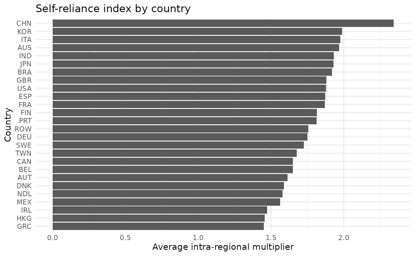

Concerning spillover to other countries, Hong Kong has the greatest value, meaning demand increases in that country triggers demand abroad. It is expected that a small city-state isn’t able to fulfill demand industry-wide, thus stimulating suppliers abroad.

ggplot(interdependence, aes(x = reorder(country, total_spillover_out), y = total_spillover_out)) +
  geom_bar(stat = "identity") +
  coord_flip() +
  labs(
    title = "Total spillover to other countries by country",
    x = "Country",
    y = "Sum of induced multipliers abroad"
  ) +
  theme_minimal()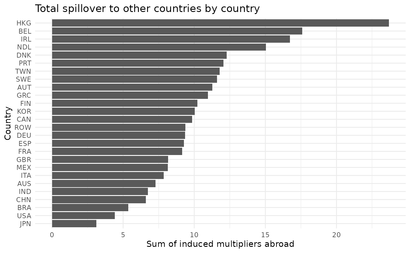

On the other hand, USA absorbs the most spillover-in effects. It means that USA benefits the most from demand shocks in other countries.

interdependence |>
  subset(!country %in% "ROW") |>
  ggplot(aes(x = reorder(country, total_spillover_in), y = total_spillover_in)) +
  geom_bar(stat = "identity") +
  coord_flip() +
  labs(
    title = "Total spillover absorbed by country",
    x = "Country",
    y = "Sum of induced multipliers at home"
  ) +
  theme_minimal()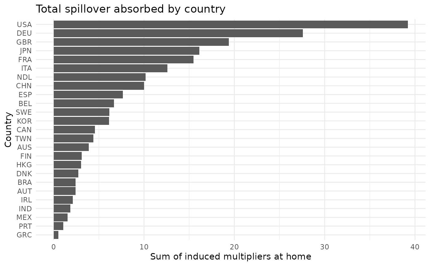

The Spillover Balance measures whether a specific region or sector is a net “giver” or a net “receiver” of economic stimulus across boundaries. It is calculated as the difference between the economic activity a region exports via spillovers and what it pulls in from others.

If balance is positive, the region is a net contributor. This means when your region spends money, it leaks a massive amount of demand out to other regions, but when they spend money, your industries don’t catch much of it.

A negative balance indicates the country is a net beneficiary, meaning your economy is highly capable of capturing the spillover effects of external spending. When other regions increase production, your local industries see a massive surge in demand for your intermediate inputs.

Results demonstrates that highly industrialized countries has negative balance, meaning they are able to absorb more spillover effects than leak it.

interdependence |>
  subset(!country %in% "ROW") |>
  ggplot(aes(x = reorder(country, spillover_balance), y = spillover_balance)) +
  geom_bar(stat = "identity") +
  coord_flip() +
  labs(
    title = "Spillover balance by country",
    x = "Country",
    y = "Spillover out - Spillover in"
  ) +
  theme_minimal()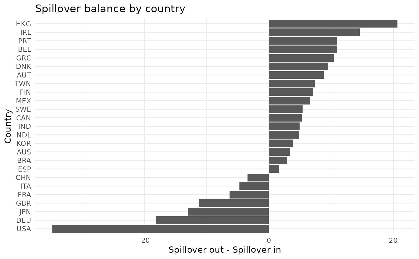

The Spillover Export Share measures the degree of external leakages relative to the total economic impact. It evaluates how much of the total economic multiplier generated by a region’s initial spending escapes to benefit foreign economies rather than staying local.

A higher share (e.g., 60%) indicates that a massive portion of the economic stimulus leaves the region. This typically happens in highly specialized, smaller, or open economies that rely heavily on importing specialized components, parts, or raw materials to complete production.

A lower share (e.g., 10%) means that the vast majority of the multiplier effect stays locked inside the domestic economy. This is characteristic of large, highly diversified economies with mature internal supply chains that can supply almost all of their own intermediate needs.

ggplot(interdependence, aes(x = reorder(country, spillover_export_share), y = spillover_export_share)) +
  geom_bar(stat = "identity") +
  coord_flip() +
  labs(
    title = "Spillover export share by country",
    x = "Country",
    y = "total_spillover_out / (out + in)"
  ) +
  theme_minimal()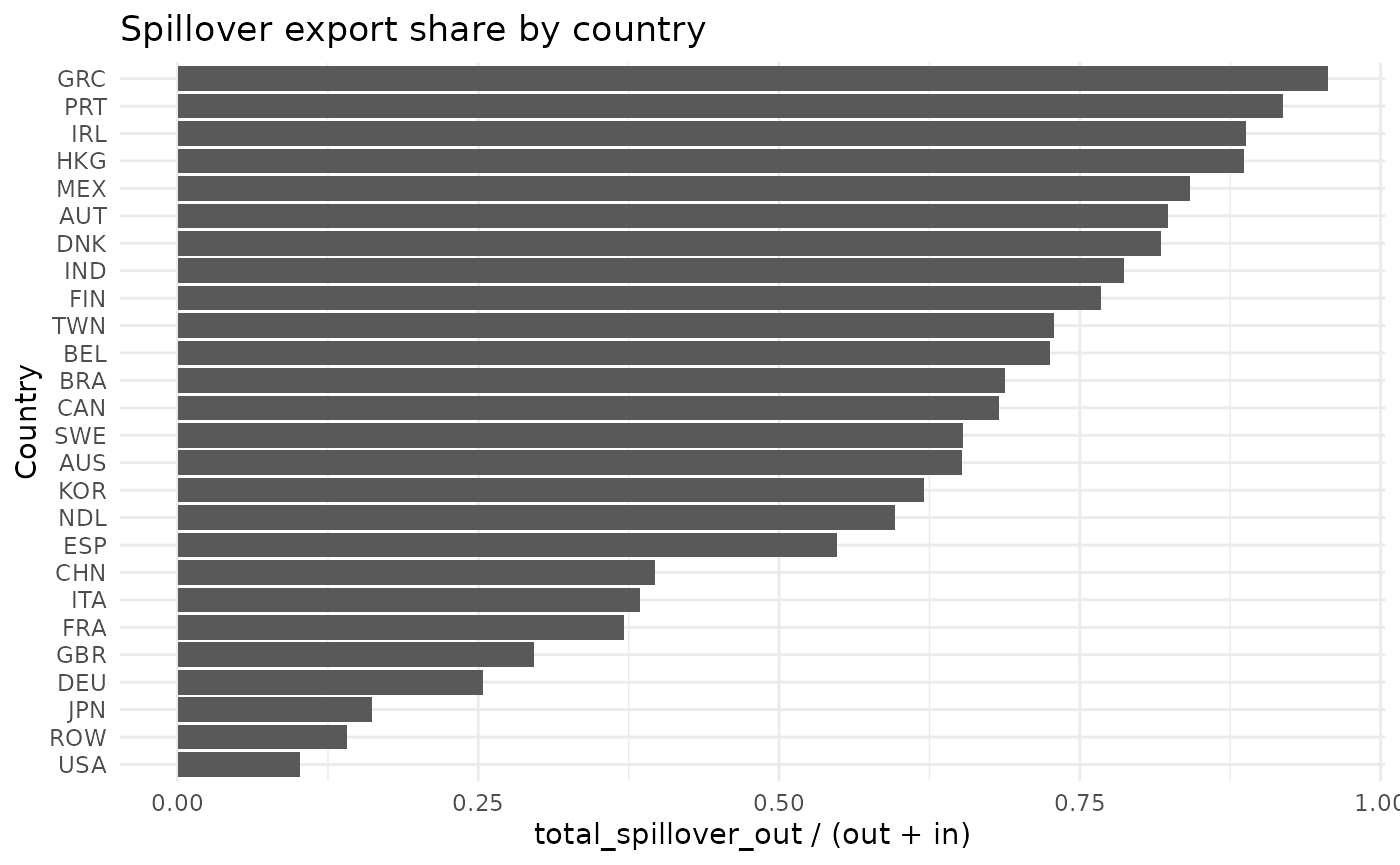

Bilateral Trade Analysis

The miom class allows extraction of bilateral trade flows between any two countries using the get_bilateral_trade() method:

# Get bilateral trade flows
trade_flow1 <- world_2000$get_bilateral_trade("BRA", "USA")
knitr::kable(trade_flow1[1:10, 1:5],
  digits = 2,
  caption = paste("Trade flows from", "BRA", "to", "USA", "(first 10 buying sectors, first 5 supplying sectors)")
)

Trade flows from BRA to USA (first 10 buying sectors, first 5 supplying sectors)
	BRA_Agriculture, Hunting, Forestry and Fishing	BRA_Mining and Quarrying	BRA_Food, Beverages and Tobacco	BRA_Textiles, leather and footwear	BRA_Pulp, paper, printing and publishing
USA_Agriculture, Hunting, Forestry and Fishing	18.23	0.02	92.85	1.80	2.80
USA_Mining and Quarrying	5.19	13.05	0.47	0.20	0.84
USA_Food, Beverages and Tobacco	8.45	0.06	29.15	1.99	0.19
USA_Textiles, leather and footwear	1.56	1.47	2.02	131.26	1.56
USA_Pulp, paper, printing and publishing	0.44	2.22	15.41	8.80	111.75
USA_Coke, refined petroleum and nuclear fuel	10.27	5.17	6.30	2.43	1.53
USA_Chemicals and chemicals products	467.80	31.80	79.89	138.63	129.08
USA_Rubber and plastics	3.79	3.62	20.65	5.88	9.43
USA_Other non-metallic mineral	0.58	1.00	2.26	0.21	0.24
USA_Basic metals and fabricated metal	2.62	11.05	13.40	1.16	4.23


trade_flow2 <- world_2000$get_bilateral_trade("USA", "BRA")
knitr::kable(trade_flow2[1:10, 1:5],
  digits = 2,
  caption = paste("Trade flows from", "USA", "to", "BRA", "(first 10 buying sectors, first 5 supplying sectors)")
)

Trade flows from USA to BRA (first 10 buying sectors, first 5 supplying sectors)
	USA_Agriculture, Hunting, Forestry and Fishing	USA_Mining and Quarrying	USA_Food, Beverages and Tobacco	USA_Textiles, leather and footwear	USA_Pulp, paper, printing and publishing
BRA_Agriculture, Hunting, Forestry and Fishing	91.70	0.08	211.27	4.86	6.39
BRA_Mining and Quarrying	1.24	20.45	0.88	0.15	1.12
BRA_Food, Beverages and Tobacco	22.36	0.12	145.10	2.35	1.80
BRA_Textiles, leather and footwear	1.94	0.19	1.02	111.85	9.46
BRA_Pulp, paper, printing and publishing	1.64	1.09	37.91	4.97	185.86
BRA_Coke, refined petroleum and nuclear fuel	36.13	19.79	8.43	3.78	15.55
BRA_Chemicals and chemicals products	44.36	12.97	18.40	52.28	48.02
BRA_Rubber and plastics	1.99	1.11	15.42	1.57	5.05
BRA_Other non-metallic mineral	0.36	3.31	12.77	2.27	1.04
BRA_Basic metals and fabricated metal	7.96	31.28	87.30	11.21	58.69

These matrices show the intermediate goods flows from the origin country (columns) to the destination country (rows) by sector. The values represent the monetary flows of intermediate inputs used in production.

Extracting Country-Specific Input-Output Tables

Lastly, one can obtain single-region iom objects from the multi-regional system. The extract_country() method allows you to extract domestic input-output tables for individual countries from the multi-regional system:

# Extract domestic economy for deutschland in the dataset
deutsch_iom <- world_2000$extract_country("DEU")

The extracted iom object contains only the domestic transactions for the specified country:

# Show a subset of the domestic intermediate transactions
knitr::kable(deutsch_iom$intermediate_transactions[1:8, 1:8],
  digits = 0,
  caption = paste("Deutschland Domestic Intermediate Transactions (first 8x8 sectors, millions USD)")
)

Deutschland Domestic Intermediate Transactions (first 8x8 sectors, millions USD)
	DEU_Agriculture, Hunting, Forestry and Fishing	DEU_Mining and Quarrying	DEU_Food, Beverages and Tobacco	DEU_Textiles, leather and footwear	DEU_Pulp, paper, printing and publishing	DEU_Coke, refined petroleum and nuclear fuel	DEU_Chemicals and chemicals products	DEU_Rubber and plastics
DEU_Agriculture, Hunting, Forestry and Fishing	1667	18	20853	247	285	10	158	160
DEU_Mining and Quarrying	37	68	52	9	42	1201	145	12
DEU_Food, Beverages and Tobacco	2655	21	9895	156	89	74	926	105
DEU_Textiles, leather and footwear	5	0	4	279	4	1	16	22
DEU_Pulp, paper, printing and publishing	74	74	1757	393	12433	117	1426	392
DEU_Coke, refined petroleum and nuclear fuel	365	31	214	62	96	799	925	100
DEU_Chemicals and chemicals products	806	68	544	871	847	292	6702	2698
DEU_Rubber and plastics	147	56	874	190	470	62	1012	2122


# Show total production
knitr::kable(t(deutsch_iom$total_production[1, 1:12]),
  digits = 0,
  caption = paste("Deutschland Total Production (first 12 sectors, millions USD)")
)

Deutschland Total Production (first 12 sectors, millions USD)
DEU_Agriculture, Hunting, Forestry and Fishing	DEU_Mining and Quarrying	DEU_Food, Beverages and Tobacco	DEU_Textiles, leather and footwear	DEU_Pulp, paper, printing and publishing	DEU_Coke, refined petroleum and nuclear fuel	DEU_Chemicals and chemicals products	DEU_Rubber and plastics	DEU_Other non-metallic mineral	DEU_Basic metals and fabricated metal	DEU_Machinery	DEU_Electrical and optical equipment
44318	11871	117494	27820	77379	35496	110737	46673	35857	135138	142012	154388

You can then perform standard input-output analysis on the domestic economy:

deutsch_iom$compute_tech_coeff()$compute_leontief_inverse()$compute_multiplier_output()

knitr::kable(head(deutsch_iom$multiplier_output, 12),
  digits = 4,
  caption = paste("Deutschland Domestic Output Multipliers (first 12 sectors)")
)

Deutschland Domestic Output Multipliers (first 12 sectors)
sector	multiplier_simple	multiplier_direct	multiplier_indirect
DEU_Agriculture, Hunting, Forestry and Fishing	1.6908	0.4146	1.2762
DEU_Mining and Quarrying	1.7559	0.4657	1.2902
DEU_Food, Beverages and Tobacco	2.0067	0.5981	1.4086
DEU_Textiles, leather and footwear	1.6419	0.3961	1.2458
DEU_Pulp, paper, printing and publishing	1.7893	0.4791	1.3102
DEU_Coke, refined petroleum and nuclear fuel	1.7602	0.4592	1.3010
DEU_Chemicals and chemicals products	1.7729	0.4766	1.2963
DEU_Rubber and plastics	1.7117	0.4319	1.2798
DEU_Other non-metallic mineral	1.7336	0.4434	1.2902
DEU_Basic metals and fabricated metal	1.7580	0.4514	1.3065
DEU_Machinery	1.7582	0.4518	1.3064
DEU_Electrical and optical equipment	1.7421	0.4492	1.2928

REFERENCES

Miller, Ronald E., and Peter D. Blair. Input-Output Analysis: Foundations and Extensions. 2nd ed. Cambridge University Press, 2009. https://doi.org/10.1017/CBO9780511626982.

June 08, 2026